 |


5. Time response analysis
|
|
|
|
5. 1 INTRODUCTION
Time response analysis of a Control system means to analyze the variation of the output of a system with respect to time. The output behavior with respect to time should be within specified limits to have satisfactory performance of the system. The complete base of stability analysis (chapter 6) lies in the time response analysis. In practical systems, abrupt changes don’t usually occur and the output takes a definite time to reach its final value. This time taken varies from system to system and depends on many factors.
The total output response can be analyzed in two separate parts. First is the part of the output during the time it takes to reach its final value. The second is the final value attained by the output, which will be close as possible to the desired value, if things go as planned.
This can be further explained by considering a practical example. Suppose we want to travel from city A to city B. It will take finite time to reach city B. This time depends on whether we travel by bus or train or plane. Similarly, whether we reach city B or not depends on number of factors like weather, condition of road etc. So in short we can classify the output as,
1. Where to reach?
2. How to reach?
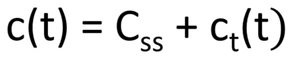
So the effectiveness and accuracy of the system depends on the final value reached by the system, which should be close to desired value as possible and also that final value should be reached in smoothest manner possible. The final value achieved by the output is called the Steady state value, while the output variations within the time taken to steady state is called the transient response of the system.
The transient response of a system is that part of the response that dies to zero after some time as the system reaches its final value. It is denoted as ct(t). Systems in which the transient response dies out after some time are called stable systems.
i. e. for stable systems,

Typically, the transient response is exponential or oscillatory in nature.

The steady state response is that part of the time response that remains after the transients have died down. It is denoted as Css. The steady state response indicates the accuracy of the system and the difference between the desired output and the actual output is known as the steady state error (ess).
Hence the total time response of the system can be written as,
5. 2 STANDARD TEST INPUTS
Usually the time response analysis of Control systems is done with the help of Standard test inputs. The evaluation of the system is done on the basis of the system response to these standard test inputs. Once the system behaves satisfactorily to these test input, its time response to the actual inputs is also assumed to be satisfactory. In practice, many signals (that are functions of time) can be used as test inputs, but the commonly used standard test inputs are:
1. Step input
Step function is mathematically defined as,
|
|
|

Step Input is like the sudden application of an input at a specified time. If A = 1, then it is called the Unit step function.
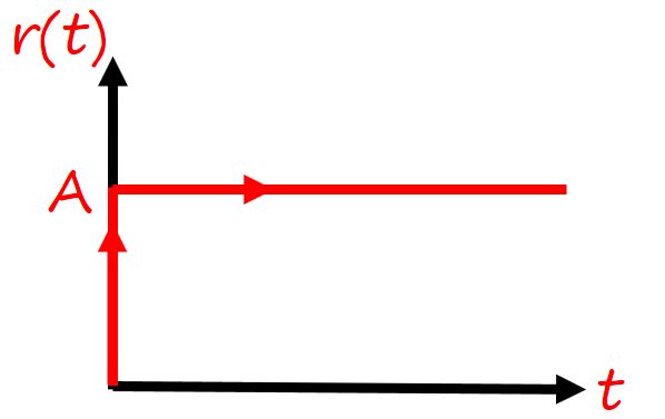
The Laplace transform of step function is A/s.
2. Ramp Input
Ramp function is mathematically defined as,

Ramp input is nothing but the gradual application of an input. If A = 1, then it is called the Unit ramp function.
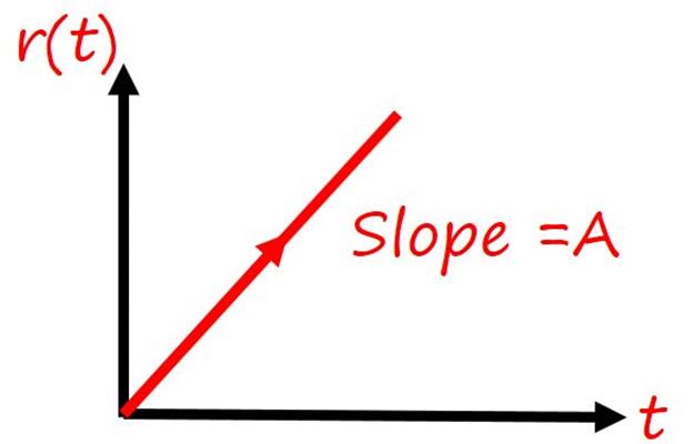
The Laplace transform of the ramp function is A/s2.
3. Parabolic Input
Parabolic function is mathematically defined as,
If A = 1, then it is called the Unit Parabolic function.

The Laplace transform of the parabolic function is A/s3.
4. Impulse Input
We have already discussed the impulse function in detail in chapter 3. Impulse function is mathematically defined as,

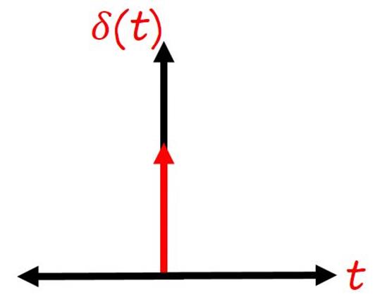
The Laplace transform of the parabolic function is 1.
5. Sinusoidal input
Sine waves and Cosines waves are collectively known as sinusoids or sinusoidal signals. Mathematically Sinusoids are mathematically represented as,


where A is the Amplitude (maximum height of the signal), ω is the angular frequency and ɸ is the phase. Sine waves and Cosines waves are basically the same, except that they start at different times (ie they are 90 degrees of phase).
Usually, the Impulse signal is used for Transient response analysis and the Steady state analysis is carried out using all the above mentioned test signals.
5. 3 FIRST ORDER SYSTEM
First order systems are those systems which can be described by first order differential equations. In First order systems the highest power of ‘s’ in the denominator of the closed loop transfer function is 1. I'm sure you've run into a fair share of first-order systems before, most popular one being the R-C filter.

Just like our RC circuit, the general form of the transfer function of First order systems is,
Where T is the time constant of the system.

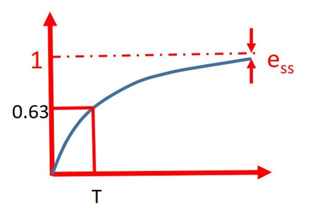
Let’s now calculate the Unit Impulse response of a first order system.

The interesting thing to note here is that the input pole at the origin is responsible for the steady state response and the system pole at s = -T is responsible for the transient response. So the transient response is totally dependent on the parameter T (Time constant). The time constant can be defined as the time taken by the step response to reach 63% of its final value.
5. 4 SECOND ORDER SYSTEM
Compared to the simplicity of a first-order system, a second-order system exhibits a wide range of responses that must be analyzed and described. Whereas varying a first-order system’s parameter simply changes the speed of the response, changes in the parameters of a second-order system can change the form of the response.
The transfer function of a 2nd order system is generally of the form,


The behavior of the second-order system can then be described in terms of two parameters: the damping ratio (  ) and the natural frequency (
  n). Every practical second order system takes a finite time to reach its steady state and during this period the system output oscillates. But practical systems have a tendency to oppose this oscillatory nature of the system, this is called Damping. A factor called the Damping ratio is used to quantify the extent of damping, a system offers. In some systems it may be so low that the oscillations sustain for a longer time. These are called Underdamped systems. While in some other systems, the damping factor maybe so high that the system output will not oscillate at all. Instead the output follows an exponential path (like first order systems). These are called Overdamped systems.
|
|
|
In systems which offer no damping at all, the output response continues to oscillate, without ever reaching a steady state value. The frequency of oscillations in such a case is called the natural frequency.

Depending on the value of , the location of the closed loop poles vary as shown in the figure below.

The under-damped case is the most important one from the application point of view since almost all real physical dynamic control systems go through oscillations before settling at the desired steady-state value. The step response of the considered second-order closed-loop system is,

Derivation (Link)
5. 5 TRANSIENT RESPONSE SPECIFICATIONS
The general under-damped step response is as shown below

The transient response characteristics of a second order system to a unit step input is specified in terms of the following time domain specifications.
1. Delay time(td): It is the time taken for the response to reach 50% of the final value for the first time.
2. Rise time(tr): It is the time taken for the response to rise from 0% to 100% for the first time.

3. Peak time(tp): It is the time taken by the response to reach its first peak value.

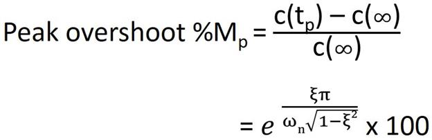
4. Peak Overshoot: It is defined as the ratio of the peak value to the final value, where the peak value is measured from the final value.
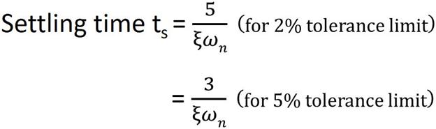
5. Settling time(ts): It is defined as the time taken by the response to reach and stay within a specified error (usually 2% or 5%)
|
|
|