 |


7. ROOT LOCUS
|
|
|
|
7. 1 CONCEPT OF ROOT LOCUS
In the previous chapters, we have seen how the location of the poles influence the stability and transient characteristics of the system. Most times one or more parameters of the system are unknown and we are unsure what the optimum values for these parameters are. So it is advantageous to know how the closed loop poles move in the system if some parameters of the system are varied. The knowledge of such movement of the closed loop poles with small changes in the system parameters greatly helps in the design of control systems.
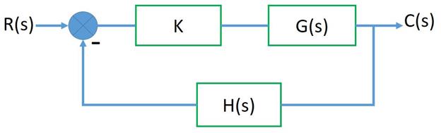
Although the Root locus can be plotted with respect to any parameter, generally the system gain K is chosen as the variable parameter. Consider the system shown below. In this system, the gain of the forward path is K G(s) and that of the feedback path is H(s).
The transfer function of this system is,

And the corresponding characteristic equation is,

It is very clear that the roots of the above equation are dependent on the values of K. Now if the gain K is varied we will get separate set of roots for the characteristic equation. The root locus is nothing but a plot showing this variation of the roots as the system gain K is varied from 0 to  .
.
7. 2 ANGLE AND MAGNITUDE CONDITION
Every point on the Root locus diagram satisfies two conditions called the Angle condition and the Magnitude condition respectively. Both the conditions can be easily obtained from the characteristic equation as follows:

8. 3 CONSTRUCTION OF ROOT LOCUS
To assist in the construction of root locus plots, the “Root Locus Rules” for plotting the loci are summarized here. These rules are based upon the interpretation of the angle condition and the analysis of the characteristic equation.
1. Rule 1 Symmetry
As all roots are either real or complex conjugate pairs so that the root locus is symmetrical to the real axis.
2. Rule 2 Number of branches
The number of branches of the root locus is equal to the number of poles P of the open-loop transfer function.
3. Rule 3 Locus start and end points
The root locus starts at finite and infinite open loop poles and it ends at finite and infinite open loop zeroes.
4. Rule 4 Real Axis Segments of Root Locus
A point on the real axis lies on the Root locus, if the sum of number of poles and zeros, on the real axis, to the right hand side of this point is odd.
5. Rule 5 Asymptotes
No. of branches of root locus approaching / terminating at infinity = no. of asymptotes = (P – Z),
where P = no. of finite open loop poles; Z = no of finite open loop zeroes.
The angle with which asymptotes approaches to infinity are called as angle of asymptotes (θ ).

6. Rule 6 Centroid
The meeting point of asymptotes is called as the centroid.

7. Rule 7 Break-in and Break-away points
Break points exists if a branch of the root locus is on the real axis between two poles or zeros. Since the root locus can only start at a pole and end at a zero, the plot breaks from the real axis to intersect with another pole or zero. If the break point lies between two successive poles, then it is called as the Breakaway Point and if the break point lies between two successive zeros, then it is called as the Breakaway Point.
|
|
|
To find these points, write k in terms of ‘s’ using the Characteristic equation. Then find the derivative of k with respect to s. The roots of equation  = 0, give the locations of break points. To differentiate between break in & break away points, find
  and substitute the values of k obtained. If > 0, then it is a break in point and if < 0, then it is a break-away point.
8. Rule 8 Intersection with the imaginary axis
The imaginary axis crossing is a point on the root locus that separates the stable operation of the system from the unstable operation. The value of ω at the axis crossing yields the frequency of oscillation. To find imaginary axis crossing, we can use the Routh-Hurwitz criterion and obtain the value of k by forcing a row of zeros in the Routh array. We can then use this value of k in the Auxiliary equation to find ‘s’ corresponding to the crossing point on the imaginary axis.
8. 4 EXAMPLE
G(s) = 
No. of poles = P = 2
No. of zeros = Z = 2
Location of Poles and Zeros:
Poles are at s = -2, s = 0. 5 and Zeros are at s = 1+2j, s = 1-2j.

Asymptotes:
Since there are equal no. of poles and zeros i. e. P-Z =0, there are no asymptotes.
Breakaway point:
Characteristic equation of the system is,
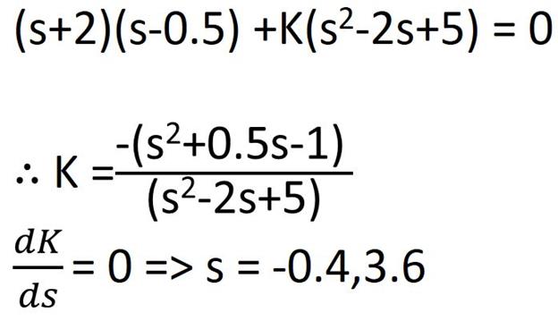
Here, since Breakaway point must lie between two consecutive poles so s = -0. 4 is a valid Breakaway Point whereas s = 3. 6 is an invalid point.
Intersection with Imaginary axis:
Routh array for the system is,

Therefore the Root Locus intersects the Imaginary axis at s =  j1. 25.

8. 5 TYPICAL ROOT LOCUS DIAGRAMS

8. 6 ROOT LOCUS IN MATLAB
Example:

Matlab Documentation for Root Locus (Link)
|
|
|