 |


Construction of the common diagnostic test Td.
|
|
|
|
Development and researching of the diagnostic tests
Aims:
1. To build the common diagnostic test for the functional-logical model.
2. To define a quotient minimal diagnostic test by the way of construction
minimization of the Boolean matrixes
3. To build the scheme of the apparatus, that investigates information logically.
4. To assemble the scheme on the laboratory table and to investigate it.
The brief theoretical information:
- Construction of the functional-logical model of the diagnosing object.
1.1 By the structural or principal scheme of the object to build the functional-logical model (FLM) in such way, that every functional element has only one exit. The quantities of the exit signals are not limited. If diagnostic object has blocks, which has K exits, you have to divide them on the K blocks with the only one exit, and to keep only that entrance, that depend on exit of this block (Fig.1).
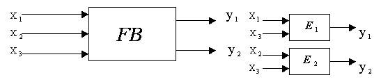 |
Fig.1. Example of breaking up of function box with two exits on the elements of functionally-logical model
1.2. To mark external exit influences and stimulate signals with the X1, X2… Xn symbols, which are given in the diagnostic of the system. To mark the exit signals of the blocks FLM by the Y1, Y2…Yn symbols.
1.3. To define the fields of the permissible and not permissible meanings for external influence and exit signals. To mark the permissible meaning with the symbol “1”, and the not permissible meaning with the symbol “0”. The not permission meanings of the exit signals lead to appearance of the not permissible signal on the exit of the element.
1.4. To consider, that the joins between the functional elements are reliable, it means, that the rejection of the system appear after the rejection of the functional elements. There is an example on the fig. 2.2.

Fig.2. The functionally-logical model of the object of the diagnostic
1.5. FLM is given by the teacher.
Construction of the matrix of condition.
For the construction of the diagnostic tests FLM can be shown by the way of matrix, which arranged connections the between the quality of conditions S and the quality of possible checking Y and quality of results of this checking’s.
The lines of the matrix mean the condition of the system Si, I = 0,n, and the columns – exit signals of the functional elements Yj, j = 0,n.
Such kinds of matrix are matrix of the condition of the object of diagnostic. The rules of construction the matrix of condition are:
1) in the case of efficient condition of the system So are all exit signals, that have permissible meanings, Yj = 1, where j = 1,n.
2) if the element E1 refuse, the exit signal of the element Ek – Yk has permissible meaning, you have to write in the check on crossing Ek and Yk symbol “1”, if it has not- permissible meaning – “0”.
In such case when all exits signals have permissible meanings, so Xi = 1, I = 1,n.
In the table 1 you can see the matrix of condition FLM, from the Fig.2.
|
|
|
Table 1
| Si | Yy1 | Yy2 | Yy3 | Yy4 | Yy5 | Yy6 | Yy7 | Yy8 | Yy9 |
| S0 | |||||||||
| S1 | |||||||||
| S2 | |||||||||
| S3 | |||||||||
| S4 | |||||||||
| S5 | |||||||||
| S6 | |||||||||
| S7 | |||||||||
| S8 | |||||||||
| S9 |
We can admit, that there is refuse of the first function element E1 (S1). In such case all exit signals of the E1, 2, 3, 4, 5 will have not- permissible meaning, so Y1 = Y2 = Y3 = Y4 = Y5 = 0. Condition of the element E6 doesn’t depend on condition of E1, because Y6 = 1. Assume, that element E2 refused we find out, that all exit signals of the E 2, 3, 5, will have not-permissible meanings, soY2 = Y3 = Y5 = 0, but Y1= Y4 = Y5 = 1.
This matrix of the condition you can use for analyse of the object of the diagnostic, that have equal characteristics of probability of refuses Q (S1) and equal values of checking exits Cyj.
Construction of the common diagnostic test Td.
Totality of checking, necessary for revelation of all conditions, which were given beforehand, is called diagnostic test (Td). With the other words, to make a diagnostic of object, is necessary to product checkings, which has the test.
For the construction of the common diagnostic test you must include neither branched exits of functional elements FLM, nor brunched external exits of the model.
Exit Ei is not-brunched, if it is joining with the only one entrance of other functional elements of model.
If exit of functional elements is not-brunched, than its condition is impossible to reveal by the meanings of the signals of other elements. Not-brunched exits (on Fig.2) are Y2, Y4, Y5, in the matrix they are Yj.
After checking of not-brunched exits it is necessary to make comparison in pairs of the lines of matrix of condition Tab. 1 on the admission of the necessary for checking exits Yj.
If in result of such comparison we find out, that all conditions have no difference in pair, the checking of such totality of exits will make the common diagnostic test – Td.
In the result of comparison of the lines of the tab. 1 we can see, that Y2, Y4, Y5 and conditions S3 and S5, S3 and S6 have the same meanings.
When we have no differences in conditions the task of finding the common diagnostic test goes to define the minimal quantity of exits Yj, and when we’ll add them to the necessary for checking exits, that can help us to differ all conditions of the system necessary for checking exits
Now, we’ll build a table, on which all lines are labelled of not-different meanings, and columns are exit signals, which are not in the totality of necessary for checking exits (Таble 2).
Таble 2
|
|
|
| Si Sk | Уy1 | Уy4 | Уy5 |
| S1 S4 | |||
| S1 S5 | |||
| S4 S5 |
If conditions, which are under comparison S and S at the exit are not the same, (1-0) or (0-1) we’ll write “1”, if they have the same meanings (0-0) or (1-1), than we’ll write “0”.
Result 1. If in this matrix is a column that has no “1”, (tab. 2.2 – columnY1) it can be delete.
Result 2. If there are series that only one “1”, these series cannot be delete, The exit Yj, will enter into the common diagnostic test.
The rule. The column (columns) of the Boolean matrix can be delete only when the matrix after deleting such columns will have one “1” in the each series.
From the matrix (tab.2) follows, that you can differ this conditions, only when you add in this test Y3 and Y6. Admit them the symbols of уj**.
So, the matrix of conditions for this case will be shown at the left part of the tab.3, and the common diagnostic test will contain: Td = { Y1, Y2, Y3, Y4, Y5, Y6}
Table 3
| Si | Yy1 | Yy2 | Yy3 | Yy4 | Yy6 | Yy7 | Yy8 | Yy9 | |
| S0 | y1^y2^y3^y4^y6^y7^y8^y9 | ||||||||
| S1 | y1^y2^y3^y4^y6^y7^y8^y9 | ||||||||
| S2 | y1^y2^y3^y4^y6^y7^y8^y9 | ||||||||
| S3 | y1^y2^y3^y4^y6^y7^y8^y9 | ||||||||
| S4 | y1^y2^y3^y4^y6^y7^y8^y9 | ||||||||
| S5 | y1^y2^y3^y4^y6^y7^y8^y9 | ||||||||
| S6 | y1^y2^y3^y4^y6^y7^y8^y9 | ||||||||
| S7 | y1^y2^y3^y4^y6^y7^y8^y9 | ||||||||
| S8 | y1^y2^y3^y4^y6^y7^y8^y9 | ||||||||
| S9 | y1^y2^y3^y4^y6^y7^y8^y9 |
4. Определение частных минимальных диагностических тестов Тimin и соответствующих им переключательных функций Si (Ti min)
Синтез алгоритма диагноза системы сводится к выбору минимального числа проверок, необходимых и достаточных для определения возможных состояний системы, т.е. к построению частных минимальных диагностических тестов Тi min  и переключательных функций Si (Timin).
Рассмотрим методику построения алгоритма. На основании минимизированной матрицы (левая часть табл. 3) можно записать переключательные функции состояний Si(Тд), . Для этого каждую строку минимизированной матрицы состояний представляют логическим произведением переменных yj, входящих в общий диагностический тест - Тд, причем над равными нулю переменными на Si - м наборе, ставится знак отрицания.
Построенная таким образом система переключательных функций Si (Тд) может быть основой для нахождения алгоритма при построении логического устройства обработки диагностической информации. Однако реализация такого алгоритма требует большого числа логических элементов, поэтому на втором этапе синтеза алгоритма логического устройства решается задача минимизации функций Si(Тд), .
|
|
|
Нахождение частных минимальных диагностических тестов Тi min и соответствующих им переключательных функций Si (Ti min) будем производить путем минимизации общего диагностического теста с помощью булевых матриц. Строками булевых матриц будут функции SiSk, полученные в результате сравнения состояний Si со всеми остальными состояниями Si,  , исключая i=k, а столбцами выходные сигналы, входящие в общий диагностический тест. Булевы матрицы для рассматриваемого примера приведены в виде таблиц (табл. 4-10)
Применяя правило и следствия минимизации булевых матриц, находим частные минимальные диагностические тесты и соответствующие им переключательные функции.
| SiSk | Y1 | Y2 | Y3 | Y4 | Y6 | Y7 | Y8 | Y9 |
| S0S1 | ||||||||
| S0S2 | ||||||||
| S0S3 | ||||||||
| S0S4 | ||||||||
| S0S5 | ||||||||
| S0S6 | ||||||||
| S0S7 | ||||||||
| S0S8 | ||||||||
| S0S9 |
T0min={y2,y3,y9},S0(T0min)=y2^y3^y9
| SiSk | Y1 | Y2 | Y3 | Y4 | Y6 | Y7 | Y8 | Y9 |
| S1S0 | ||||||||
| S1S2 | ||||||||
| S1S3 | ||||||||
| S1S4 | ||||||||
| S1S5 | ||||||||
| S1S6 | ||||||||
| S1S7 | ||||||||
| S1S8 | ||||||||
| S1S9 |
T1min={y1},S1(T1min)=y1
| SiSk | Y1 | Y2 | Y3 | Y4 | Y6 | Y7 | Y8 | Y9 |
| S2S0 | ||||||||
| S2S1 | ||||||||
| S2S3 | ||||||||
| S2S4 | ||||||||
| S2S5 | ||||||||
| S2S6 | ||||||||
| S2S7 | ||||||||
| S2S8 | ||||||||
| S2S9 |
|
|
|
T2{y1,y2},S2(T2min)=y1^y2
| SiSk | Y1 | Y2 | Y3 | Y4 | Y6 | Y7 | Y8 | Y9 |
| S3S0 | ||||||||
| S3S1 | ||||||||
| S3S2 | ||||||||
| S3S4 | ||||||||
| S3S5 | ||||||||
| S3S6 | ||||||||
| S3S7 | ||||||||
| S3S8 | ||||||||
| S3S9 |
T3min={y2,y3,y9},S3(T3min)=y2^y3^y9
| SiSk | Y1 | Y2 | Y3 | Y4 | Y6 | Y7 | Y8 | Y9 |
| S4S0 | ||||||||
| S4S1 | ||||||||
| S4S2 | ||||||||
| S4S3 | ||||||||
| S4S5 | ||||||||
| S4S6 | ||||||||
| S4S7 | ||||||||
| S4S8 | ||||||||
| S4S9 |
T4min={y1,y2,y4},S4(T4min)=y1^y2^y4
| SiSk | Y1 | Y2 | Y3 | Y4 | Y6 | Y7 | Y8 | Y9 |
| S5S0 | ||||||||
| S5S1 | ||||||||
| S5S2 | ||||||||
| S5S3 | ||||||||
| S5S4 | ||||||||
| S5S6 | ||||||||
| S5S7 | ||||||||
| S5S8 | ||||||||
| S5S9 |
T5min={y6,y7,y8},S5(T5min)=y6^y7^y8
| SiSk | Y1 | Y2 | Y3 | Y4 | Y6 | Y7 | Y8 | Y9 |
| S6S0 | ||||||||
| S6S1 | ||||||||
| S6S2 | ||||||||
| S6S3 | ||||||||
| S6S4 | ||||||||
| S6S5 | ||||||||
| S6S7 | ||||||||
| S6S8 | ||||||||
| S6S9 |
T6min={y6,y7,y8},S6(T6min)=y6^y7^y8
| SiSk | Y1 | Y2 | Y3 | Y4 | Y6 | Y7 | Y8 | Y9 |
| S7S0 | ||||||||
| S7S1 | ||||||||
| S7S2 | ||||||||
| S7S3 | ||||||||
| S7S4 | ||||||||
| S7S5 | ||||||||
| S7S6 | ||||||||
| S7S8 | ||||||||
| S7S9 |
T7min={y6,y7},S7(T7min)=y6^y7
| SiSk | Y1 | Y2 | Y3 | Y4 | Y6 | Y7 | Y8 | Y9 |
| S8S0 | ||||||||
| S8S1 | ||||||||
| S8S2 | ||||||||
| S8S3 | ||||||||
| S8S4 | ||||||||
| S8S5 | ||||||||
| S8S6 | ||||||||
| S8S7 | ||||||||
| S8S9 |
T8min={y3,y6,y7,y8},S8(T8min)=y3^y6^y7^y8
|
|
|
| SiSk | Y1 | Y2 | Y3 | Y4 | Y6 | Y7 | Y8 | Y9 |
| S9S0 | ||||||||
| S9S1 | ||||||||
| S9S2 | ||||||||
| S9S3 | ||||||||
| S9S4 | ||||||||
| S9S5 | ||||||||
| S9S6 | ||||||||
| S9S7 | ||||||||
| S9S8 |
T9min={y6,y8,y9},S9(T9min)=y6^y8^y9
Так, для матрицы, представленной табл. 4, минимальный диагностический тест mi, а соответствующая ему переключательная функция  . Значение переменной yj или
  в найденной переключательной функции для данного состояния берут из табл. 2.3: Для булевой матрицы (табл. 2.5) минимальный диагностический тест и переключательная функция:
 etc.
etc.
|
|
|