 |


Table of Contents. Preface. 1. Introduction
|
|
|
|
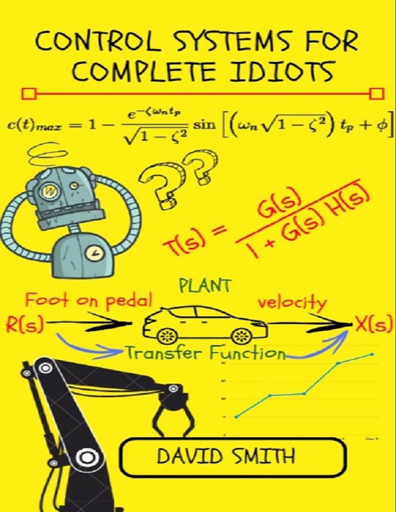
Table of Contents
PREFACE
1. INTRODUCTION
2. LAPLACE TRANSFORM
3. TRANSFER FUNCTION
4. REPRESENTATION
5. TIME RESPONSE ANALYSIS
6. STABILITY
7. ROOT LOCUS
8. FREQUENCY DOMAIN ANALYSIS
APPENDIX
REFERENCES
CONTACT
Control Systems for Complete Idiots
by David Smith
All Rights Reserved. No part of this publication may be reproduced in any form or by any means, including scanning, photocopying, or otherwise without prior written permission of the copyright holder. Copyright © 2018
Other books in the Series:
Arduino for Complete Idiots
Digital Signal Processing for Complete Idiots
Circuit Analysis for Complete Idiots
Basic Electronics for Complete Idiots
Electromagnetic Theory for Complete Idiots
Digital Electronics for Complete Idiots
Table of Contents
PREFACE
1. INTRODUCTION
2. LAPLACE TRANSFORM
3. TRANSFER FUNCTION
4. REPRESENTATION
5. TIME RESPONSE ANALYSIS
6. STABILITY
7. ROOT LOCUS
8. FREQUENCY DOMAIN ANALYSIS
APPENDIX
REFERENCES
CONTACT
PREFACE
In this day and age everything around us is automatic and our desire to automate more stuff is only increasing. Control systems finds its applications in everything you can possibly think of. The concept of Control system plays an important role in the working of, everything from home appliances to guided missiles to self-driving cars. These are just the examples of Control systems we create. Control systems also exist in nature. Within our own body, there are numerous control systems, such as the pancreas, which regulate our blood sugar. In the most abstract sense it is possible to consider every physical object a control system. Hence from an engineering perspective, it is absolutely crucial to be familiar with the analysis and designing methods of such Control systems. Control systems is one of those subjects that go beyond a particular branch of engineering. Control systems find its application in Mechanical, Electrical, Electronics, Civil Engineering and many other branches of engineering. Although this book is written in an Electrical engineering context, we are sure that others can also easily follow the topics and learn a thing or two about Control systems.
In this book we provide a concise introduction into classical Control theory. A basic knowledge of Calculus and some Physics are the only prerequisites required to follow the topics discussed in the book. In this book, We've tried to explain the various fundamental concepts of Control Theory in an intuitive manner with minimum math. Also, We've tried to connect the various topics with real life situations wherever possible. This way even first timers can learn the basics of Control systems with minimum effort. Hopefully the students will enjoy this different approach to Control Systems. The various concepts of the subject are arranged logically and explained in a simple reader-friendly language with MATLAB examples.
|
|
|
This book is not meant to be a replacement for those standard Control systems textbooks, rather this book should be viewed as an introductory text for beginners to come in grips with advanced level topics covered in those books. This book will hopefully serve as inspiration to learn Control systems in greater depths.
Readers are welcome to give constructive suggestions for the improvement of the book and please do leave a review.
1. INTRODUCTION
1. 1 INTRODUCTION
In this day and age everything around us is automatic and our desire to automate more stuff is only increasing. Control systems finds its applications in everything you can possibly think of. The concept of Control system plays an important role in the working of, everything from home appliances to guided missiles to self-driving cars. These are just the examples of Control systems we create. Control systems also exist in nature. Within our own body, there are numerous control systems, such as the pancreas, which regulate our blood sugar. In the most abstract sense it is possible to consider every physical object a control system. Hence from an engineering perspective, it is absolutely crucial to be familiar with the analysis and designing methods of such Control systems.
1. 2 TERMS
So far we have used the term “Control system” many a times. To understand the meaning of the word Control system, first we will define the word system and then we will define a Control system.
A system is nothing but an arrangement of physical components which act together as a unit to achieve a certain objective. A room with furniture, fans, lighting etc. is an example of a system. To control means to regulate or direct. Hence a Control system is an arrangement of physical components connected in such a manner to direct or regulate itself or another system. For example, if a lamp is switched ON or OFF using a switch, the entire system can be called a Control system. In short, a Control system is in the broadest sense, an interconnection of physical components to provide a desired function, involving some kind of controlling action in it.
For each system, there is an excitation and a response or to simply put it, an input and an output. The Input is the stimulus, excitation or command applied to a Control system to produce a specific response and the Output is the actual response obtained from the Control system. It may or may not be equal to the response we intended to produce from the input provided (That’s whole other story). Now consider an example, when you clap your hands, it makes sound, this is a system. So what are the input and output of this system?? Is the input, the motion of your hands?? Or Is it the trigger from your brain or something else. Similarly, what is the output of the system?? The sound?? Or the vibrations generated?? For a system, the inputs and outputs can have many different forms. In fact, it’s completely up to us to decide what a systems input and output parameters should be, based on the application and most times, Control systems have more than one input or output.
The purpose of the control system usually identifies or defines the output and input. If the output and input are given, it is possible to identify and define the nature of the system components. Fortunately for us, more often than not, all inputs and outputs are well defined by the system description. Sometimes they are not, like noises or disturbances in the output. Disturbance is any signal that adversely effects the output of a system. Some of these disturbances are internally generated, others from outside the system.
|
|
|
1. 3 CLASSIFICATION OF CONTROL SYSTEMS
There are a lot of ways to classify Control systems, Natural-Manmade, Single input single output -Single input multiple output etc., but we will focus on some of the important classifications:
1. 3. 1 Time Varying and Time Invariant Systems
Time Invariant Control systems are those in which the system parameters are independent of time. In other words, the system behavior doesn't change with time. For example, consider an electrical network, say your mobile charger, consisting of resistors and capacitors. It produces an output of 5V when connected to a 230V AC supply. This system is a time invariant one, because it is expected to behave exactly the same way, whether it’s used at 6 pm or 11 pm or any other time.
On the other hand, Systems whose parameters are functions of time are called Time varying systems. The behavior of such systems not only depends on the input, but also the time at which the input is applied. The complexity of design increases considerably for such type of Control systems.
1. 3. 2 Linear and Non-Linear Systems
A Linear system is one that obeys the Superposition property. Superposition property is a basically a combination of 2 system properties:
1. Additivity property: A system is said to be additive if the response of a system when 2 or more inputs are applied together is equal to the sum of responses when the signals are applied individually. Suppose we provide an input (x1) to a system and we measure its response. Next, we provide a second input (x2) and measure its response. Then, we provide the sum of the two inputs x1 + x2. If the system is linear, then the measured response will be just the sum of the responses, we noted down while providing the two inputs separately.
i. e. if x1(t) → y1(t) and x2(t) → y2(t),
Then the system is additive if, x1(t) + x2(t) → y1(t) + y2(t)
2. Homogeneity or Scaling property: A system is said to obey Homogeneity property, if the response of a system to a scaled input is the scaled version of the response to the unscaled input. This means that, as we increase the strength of a simple input to a linear system, say we double it, then the output strength will also be doubled. For example, if a person's voice becomes twice as loud, the ear should respond twice as much if it's a linear system.
if x(t) → y(t), then the system obeys homogeneity, if a x(t) → a y(t), where a is constant.
Combining both these properties we get the superposition property.
a x1(t) + b x2(t) → a y1(t) + b y2(t)
An interesting observation to be made from this property is that, for linear systems zero input yields zero output (assume a = 0, then output is zero).
Both Linear and Time Invariant systems are two very important classes of Control Systems. In practice, it is difficult to find a perfectly linear time invariant system. Most of the practical systems are non-linear to a certain extent. However, more often than not, we model real world systems as Linear Time Invariant systems or LTI systems. This is because, analyzing and finding solutions to non-linear time variant systems are extremely difficult and time consuming. But if the presence of certain non-linearity is negligible and not effecting the system response badly, they can be treated as Linear (for limited range of operation) by making some assumptions and approximations. This makes the math a lot easier and allows us to use more mathematical tools for analysis or in Richard Feynman's words " Linear systems are important because we can solve them". The advantages of making this approximation is far greater than any disadvantages that arises from the assumption. We will be dealing with LTI systems from this point on.
|
|
|
1. 3. 3 Continuous time and Discrete time Systems
Mathematical functions are of two basic types, Continuous functions and Discrete functions. Continuous time functions are those functions that are defined for every instant of time. This means that you can draw a continuous function without lifting your pen or pencil from the paper. Discrete time functions on the other hand, are those functions, whose values are defined only for certain instants of time. For example, if you take the temperature reading of your room after every hour and plot it, what you get is a discrete time function. The temperature values are only defined at the hour marks and not for the entire duration of time. The value of temperature at other instants (say at half or quarter hour marks) are simply not defined.
In a continuous-time Control system all the system variables are continuous time functions. In a discrete-time Control system at least one of the system variables is a discrete function. Microprocessor and computer based systems are discrete time systems.
1. 3. 4 Open and Closed Loop Systems
This is another very important classification of control systems and the features of both these types are discussed in detail in the coming sections.
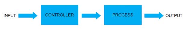
1. 4 OPEN LOOP SYSTEM
Open loop system is a system in which output or rather the variation in output has no bearing on the controlling action. In other words, in an Open loop system, the output is neither measured nor fed back for comparison with the input. This simply means that, in an Open loop system there is no mechanism to correct the output if it goes out of track. Thus the accuracy of the output in an Open loop system is completely dependent on the accuracy of the input we provide and the calibration of the system. The Open loop control systems have a major drawback; the output of the system is adversely effected the presence of disturbances. This is because the changes in the output due to disturbances are not followed by changes in the input to correct the output. So any necessary changes, need to be made manually and since the nature of disturbances aren’t the same always, it is quite difficult to maintain the accuracy in the output.
Due to these reasons, the practical applications of Open loop control systems are minimal and used only in places where the input-output relation is quite clear and the disturbances (internal and external) are minimum.
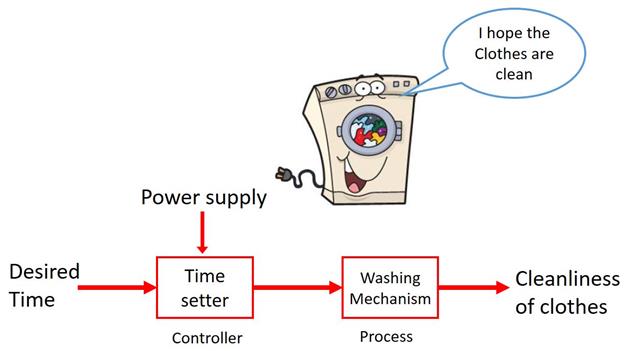
One good example of a practical Open loop system is your washing machine. Soaking, washing, rinsing in the washing machine operate on a time basis. The machine does not measure the output i. e. the cleanliness of the clothes (at least not the ordinary ones).
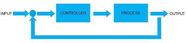
1. 5 CLOSED LOOP SYSTEM
A Closed loop system is a system in which the variations in the output has a bearing on the control mechanism of the system. In a Closed loop system, an actuating error signal, which is the difference between the input signal and the output signal (in some form, not always directly), is fed to the controller. It is this error signal that drives the system. If the output of the system falls lower than the desired value, the corresponding error signal ensures that the output rises to the desired value and if the output rises above the desired value, its corresponding error signal makes the output decrease to the desired value. This way the output is always scrutinized and the corrections are made automatically. Doesn’t Closed loop systems already seem more useful??
|
|
|
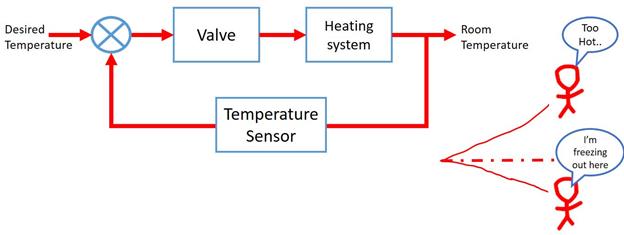
A Home heating system is an example of a Closed loop system. When the temperature is above the desired value, an error signal is generated and the valve is actuated to bring the temperature down to desired value. Similarly, it automatically raises the temperature, when it’s too cold.
Something to be noted is that, it is not always possible, sometimes not desirable, to feed back the available output signal directly. Depending on the nature of the controller and the plant, it may be required to attenuate it, amplify it, or sometimes even change its nature (to digital etc. ). This changed input is called the reference input. While the Closed loop systems have much more desirable properties than its counterpart, they do have some undesirable properties. Firstly, with all the complexity, designing these systems is a challenge in itself. But the critical area where they lose out to the Open loop systems is stability. That’s a bit odd, isn’t it?? One might have figured, that with the self-correcting nature of these systems, they are far more stable. The problem is that these systems have a tendency to over correct the errors and that may overtime lead to oscillations. The problem of stability is a severe one and must be taken care of in the design stages (which again adds complexity in designing).
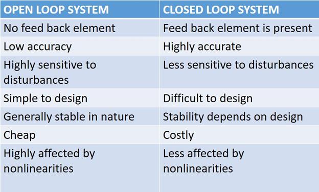
1. 6 OPEN LOOP V/S CLOSED LOOP SYSTEM
|
|
|