 |


3. Transfer function
|
|
|
|
3. 1 CONCEPT
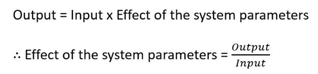
A Transfer function is nothing but a mathematical indication of the relationship existing between the input and the output of a Control system. In other words, the transfer function is a mathematical expression that tells what the system is doing with our input. In designing a system, first the system parameters are designed and their values are chosen as per requirement. Then we provide an input and see the performance of the system. We can roughly say that the output of the system is the product of the input and effect of the system parameters. Therefore, the effect of the system parameters can be expressed as the ratio of the Output to the Input. Due to the characteristics of system parameters, the input gets transferred into output, once applied to the system. This is the concept of Transfer function.
Mathematically, the Transfer function is defined as the ratio of Laplace transform of the output of the system to the Laplace transform of the input of the system, assuming zero initial conditions.

The Transfer function of the system G(s) is given by,

The reason we consider the Transfer function in the Laplace domain will become clear in the next section. For now, just understand that the Transfer function is a function of ‘s’.
(ex) G(s) = 
The following example will make the concept of Transfer function clear: Suppose you are asked to write your name on a black board. But there’s a catch, you can’t do this directly, instead you have to use a contraption, as shown below.

Is this even possible??, you must be thinking. I can totally understand your skepticism, for a system with these many transformations, drawing a straight line would be a challenge, let alone something as complex as your name. Disregarding its complexity, this is nothing but another Control system with an input and an output. The difference here is that this Control system is itself made up of 4 other Control systems. So to understand the effect of the Control system as a whole, we need to characterize the behavior of each part separately and combine them. It may seem like a lot of effort, but it’s not. All we have to do is to find the transfer function of each part and combine them in some manner. Since the output of one part is the input to the next part, the Transfer function of the system as a whole is simply the product of individual Transfer functions.

3. 2 UNIT IMPULSE FUNCTION
The Unit Impulse function is a very important function in Control systems and Signal Processing. Mathematically, it is defined as:

Think of the Impulse signal like a short pulse, like the output when a switch is turned on and off as fast as you can. But, if the value of the Unit Impulse function is ∞ at t = 0, then why the name Unit Impulse function?? The name comes from the fact that the Unit impulse function has a unit area at t =0. Consider a narrow rectangular pulse of width A and height 1/A, so that the area under the pulse = 1. Now if we go on reducing the width A and maintain the area as unity, then the height 1/A will go on increasing. Ultimately when A  0, 1/A
  and it results in a pulse of infinite magnitude. It is very clear from this, that the Unit impulse function has infinite magnitude at t = 0.
|
|
|


The height of the arrow is used to depict the area of a scaled impulse. The unit Impulse function is also known as the delta function or the delta-dirac function.
The obvious question that may come to your mind at this point is, “What is so special about the Unit Impulse function? ”. The answer to that lies in the figures shown below.

Figured it out yet? In the second figure shown above, we have substituted the signal in the first figure, by infinite number of Impulses of appropriate magnitudes at each instant of time. In this manner, any signal can be constructed out of scaled and shifted Unit Impulse signals. This is called the Sifting property of Unit Impulse function. This may not seem like a big deal, but trust me it is.
3. 3 IMPULSE RESPONSE
When working with a control system, we would want to test out its response to a signal or a range of signals. How do we do that? Surely, we can't go around testing the response of every signal one after the other. It's too cumbersome and most times uneconomical. There's got to be an easier way. Actually there is, in the last section, we saw how a signal can be expressed as the sum of appropriately scaled and shifted Unit Impulses. We can put that property to good use. By figuring out how the system responds to a Unit Impulse signal, we can predict the system response to any input signal. The response of a system to a Unit Impulse signal is called the Unit Impulse Response (denoted by h(t)).

Because these are LTI systems, the Impulse response is scaled and shifted by the same factor as the input Impulse signal. So the system response to any input can be obtained by summing up the scaled and shifted impulse responses (as shown in above figure).
But since summing up infinite impulse responses isn’t possible, mathematicians came up with what is known as the Convolution integral (denoted by * operator).

Woah!! That seems awfully hard. Fortunately for us, the convolution integral corresponds to simple multiplication in the Laplace domain (told ya Laplace would come in handy).
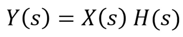
Where H(s) is the Unit Impulse response in the Laplace domain, which by the way is the Transfer function of the system.
3. 4 TERMINOLOGIES RELATED TO TRANSFER FUNCTION
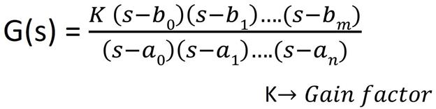
The Transfer function of a system can expressed as the ratio of two functions of ‘s’, G(s) =  . In most cases, it is more convenient to represent the rational transfer function in the factorized form.
3. 4. 1 DC Gain
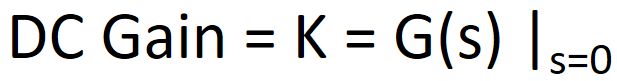
The term K in the transfer function (in factorized form) is called the Gain factor or the DC gain. It is simply the value of the transfer function at zero frequency i. e. s=0.
3. 4. 2 Poles & Zeros
The values of ‘s’ for which the magnitude of the transfer function becomes infinity are called the Poles of the system. These are nothing but the roots of the equation obtained after equating the denominator of the transfer function to zero.
|
|
|
And the values of ‘s’ for which the magnitude of the transfer function becomes zero are called the Zeros of the system. Poles and Zeros may be real or complex-conjugates or combination of both.
(ex) G(s) = 
For this transfer function, there are two poles at s= 0 and s= -5 and a zero at s= -2. These values can be plotted on the complex s-plane, using an X for poles and O for zeros.

3. 4. 3 Order of the System
The order of the system is the highest power of ‘s’ present in the denominator polynomial of the transfer function. The system in our last example is a second order system.
|
|
|