 |


2. Laplace transform
|
|
|
|
2. 1 INTRODUCTION
Like any other engineering subject, Control systems has its fair share of math, but at the same time it isn’t anywhere as math intensive as say, DSP is or EM theory is. In control systems, we are mainly dealing with Laplace transform and its discrete version, z- transform (for discrete Control systems).
You know, it’s always a little scary when we devote a whole chapter just for a Math topic. Laplace transforms (or just transforms) can seem scary at first. However, as we will see, they aren’t as bad as they may appear at first. To be honest, only the application part of Laplace transform is relevant to us, as far Control systems is concerned. Just the ability is to use the Laplace operator is more than enough. But just for completeness of the topic and considering how useful a tool it is, we will try and explain the concept and develop an intuitive understanding about the Laplace transform.
2. 2 CONCEPT
The Laplace transform is a well-established mathematical technique for solving differential equations. It is named in honor of the great French mathematician, Pierre Simon De Laplace (1749-1827). Like all transforms, the Laplace transform changes one signal into another according to some fixed set of rules or equations. WAIT…. did I say signals? That’s right, here by signals we mean a continuous function (of time mostly) and also, it is the more appropriate term in an electrical engineering context.
Before we dig into Laplace transform, let’s look into transforms in general. So what is a transform? Why do we need them?
Let’s begin by considering a simple computational problem: compute the value of x = 3. 42. 4. It is not easy to get the exact value using straightforward methods. What we can do to make this problem solvable is to take natural log on both sides: now the equation becomes ln(x) = 2. 4 ln (3. 4). Now the value of ln(x) can be easily obtained and to obtain the value of x, all we have to do is to take the antilog of the value obtained. What we did was to take the hard problem, convert it into an easier equivalent problem. This is the very idea behind transforms. The concept of transformation can be illustrated with the simple diagram below:
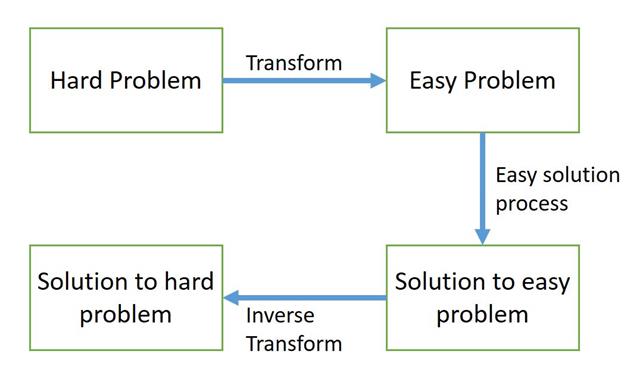
The peculiarity of physical systems (LTI systems) are that they can be modeled by Differential equations. But solving Differential equations isn’t the easiest of tasks. What kind of transformation might we use with ODEs? Based on our experience with logarithms, the dream would be a transformation, which allows us to replace the operation of differentiation by some easier operation, perhaps something similar to multiplication. Even if we don’t get this exactly, coming close might still be useful. This is exactly what the Laplace transform is used for. The Laplace transform, transforms the differential equations into algebraic equations which are easier to manipulate and solve. Once the solution in the Laplace transform domain is obtained, the inverse Laplace transform is used to obtain the solution to the differential equation.
|
|
|
The Laplace transform of a function f(t), denoted as F(s), is defined as:
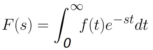
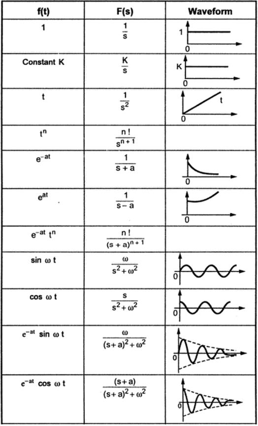
Yes, I know this equation looks menacing at first glance. But fortunately, most times you don’t need to use this equation, you can easily get away with knowing some standard results.
2. 3 PHYSICAL MEANING
Making sense of the Laplace transform and getting your head around its physical meaning isn’t the easiest of tasks. To understand the meaning of Laplace transform you need to have some idea about the Fourier transform (Link). If you look at Fourier transform equation, you can spot a striking similarity with the Laplace transform equation. The two equations are very similar, except that in the Laplace transform equation, term ‘s’ is used in place of ‘j  ’. This similarity is because the Laplace transform was developed in order to overcome some limitations of the Fourier transform. From a mathematical standpoint, the Fourier transform is a subset of the Laplace transform. The connection between the two will become more apparent as we write the expansion of ‘s’,
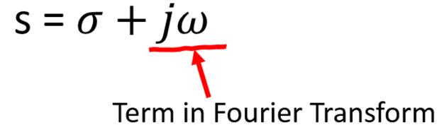
Where  is a real number.
The Laplace transform is basically the Fourier transform with an additional term (  ). Although the Fourier transform is an extremely useful tool for analyzing many kinds of systems it has some shortcomings that can be overcome, in many ways, by the Laplace Transform. In particular, the Fourier transform is not very useful for studying the stability of systems because, in studying instabilities, it is often necessary to deal with signals that diverge in time. We know that the Fourier integral does not converge for signals that diverge because such signals are not absolutely integrable.
Because of the exponential weighting, the Laplace transform can converge for signals for which the Fourier transform does not converge. Depending upon the value of σ, which is the real part of s, a signal (whose transform we are taking) is be multiplied by a decaying or expanding exponential. By tacitly choosing the value of σ, thereby multiplying the signal with a decaying exponential, we can ensure that it becomes convergent. The region in the “s” plane where this infinite integral converges is called the region of convergence (ROC).
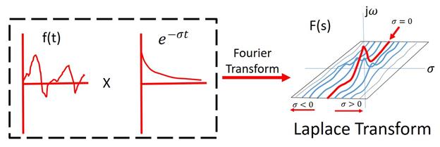
Intuitively, this means that the Laplace transform analyses the signals both in terms of exponentials and sinusoids, just as the Fourier transform analyses signals in terms of sinusoids. The center line in the s-plane (at = 0) corresponds to the Fourier.
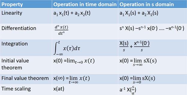
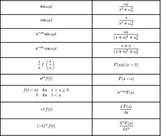
2. 4 PROPERTIES OF LAPLACE TRANSFORM
Some of the basic properties of Laplace transform,
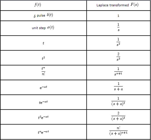
2. 5 STANDARD LAPLACE TRANSFORM PAIRS
2. 6 INVERSE LAPLACE TRANSFORM
Finding the Inverse Laplace transforms of functions isn’t terribly difficult. Most times Inverse Laplace transforms of functions can be figured out by inspection. The general method to find the Inverse Laplace transforms of functions is to express them as partial fractions and then make it into a convenient form and figure out which function’s Laplace each term is. The table below shows some basic Laplace inverse pairs.
2. 7 SOLVING DIFFERENTIAL EQUATIONS
|
|
|
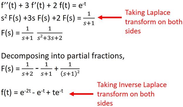
As mentioned earlier, one of the biggest uses of Laplace transform is in solving differential equations. The procedure is best illustrated with an example.
Example:
f ’’(t) + 3 f’(t) + 2 f(t) = e-t, with the initial conditions f(0) = f’(0) =0
More Examples (Link)
|
|
|